NPB 163/PSC 128

Simulating differential equations

Discrete-time systems

• In most real physical systems, such as neurons, time is continuous. Thus, we use mathematical constructs such as and to represent summation and differences over continuous time, which is infinitely divisible.
  
  
• If we wish to simulate such systems on a digital computer, then we have no choice but to discretize time. Note however that this is not true of all computation in general. Analog computers, which pre-dated the digital computers we have today, serve as very useful simulation tools for studying complex dynamical systems using op-amps and capacitors without the need to discretize time.
  
  
• In the digital computer, we represent the continuous-time signal by sampling at discrete points in time:
                   
  
  where is the sampling interval and n is the sample number (an integer). Thus, represents a sample of at time . Note that the sampling interval must be picked sufficiently small so as to capture the significant time-varying structure in , otherwise aliasing will result (this is what makes wagon wheels and propellers look like they’re sometimes moving backwards in movies).
  
  

• A discrete-time approximation to the derivative is computed by taking the difference between adjacent samples divided by the sampling interval:
  
                     
  
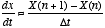
  In the limit as , this relationship becomes an equality (by definition).
  
  
• Now lets say we wish to simulate the differential equation . Re-expressing this as a discrete-time difference equation, we have
  
                      .
  
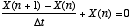  With a little algebraic manipulation of terms, we obtain
  
                     
  
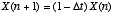
  Thus, to simulate this system on a computer, we simply run a loop for and set X to a fraction of its previous value at each iteration. Note however that if we pick too large, then the system will not decay to zero but rather explode to . In this case, we must have <1 since .
  
  
• In a similar fashion, we can simulate the leaky-integrator with time-constant
  
                       
  
  via the difference equation
  
                   
  
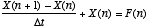
  which results in the discete-time equation
  
                   
  
  where and . Note again though that in order for this simulation to work we must have , and so must be picked to be small relative to .
  
  
• The discete-time version of the leaky integrator gives us another perspective on what it is computing. Here we see that at each time step, the next value of X is a weighted sum of the current value of X and the current value of the input F. The weights that are used to combine X and F add to one. Thus, if then the next value of X is 90% of its current value plus 10% of the current value of F. It is easy to show that this recursive computation is equivalent to taking an expontentially decaying weighted sum of the present and past values of F.
  
  
• This method of simulating a differential equation is known as Euler’s method. It is by far the simplest method of simulating a differential equation. Its disadvantage though is that it only crudely approximates the derivative, and so must be picked very small to obtain accurate simulations. A small means that many iterations are required, which demands more time. More efficient methods for simulating differential equations, such as the Runge-Kutta method, achieve the same degree of accuracy with larger time steps and hence fewer iterations.